Processing BOLD Data
Scenario: You’ve collected some BOLD data and you’re interested in functional connectivity.
This example will walk you through the typical functional connectivity pipeline in the 4dfp suite - generic BOLD pre-processing, fcMRI pre-processing, and seed-based correlation.
System requirements
These scripts assume that the current shell is csh. To check/change your shell you can use the following commands:
# output the current shell
echo $0

# switch to csh shell
csh
They also expect REFDIR to be set as an environment variable, so you will need to add it to your login script:
setenv REFDIR /data/petsun43/data1/atlas
Additionally, the scripts rely on a couple external programs that will need to be on your system path.
First, check if mri_convert and mcverter are on your path:
which mri_convert
which mcverter
If either program is not found, you will need to add the following lines to your login script.
set path = ( $path \
             $FREESURFER_HOME/bin \
             /data/nil-bluearc/hershey/unix/software/MRIConvert/MRIConvert-2.1.0/usr/bin \
           )
Preparing DICOM data
If you haven’t already downloaded your data, see Downloading data from CNDA.
Once you have DICOM data downloaded and transferred to your project directory, you will start by sorting your DICOM data.
How to run this will depend on the DICOM directory structure.
In the following examples we’ll use NEWT002_s1 for an example MR session,
and assume that the DICOM data is under the SCANS/ directory:
$ cd /path/to/project
$ cd NEWT002_s1
$ ls
SCANS

$ ls SCANS
If SCANS/ contains a flat list of DICOMs, you will use dcm_sort:
$ dcm_sort SCANS
If SCANS/ contains numbered directories, you will use pseudo_dcm_sort.csh:
$ pseudo_dcm_sort.csh SCANS
This will create study folders for each of the scans downloaded from CNDA, as well as a SCANS.studies.txt file that
contains the mapping of study number to series description
$ ls
SCANS               study10     study21     study25     study29
SCANS.studies.txt   study14     study23     study27

$ cat SCANS.studies.txt
10   tfl3d1_16ns    ABCD_T1w_MPR_vNav                                   176
14   spc_314ns      ABCD_T2w_SPC_vNav                                   176
21   epse2d1_90     SpinEchoFieldMap_AP_2p4mm_64sl                        3
23   epse2d1_90     SpinEchoFieldMap_PA_2p4mm_64sl                        3
25   epfid2d1_90    fMRI_AP_2p4mm_MB4_tr1230_te33                       250
27   epfid2d1_90    fMRI_AP_2p4mm_MB4_tr1230_te33                       250
29   epfid2d1_90    fMRI_AP_2p4mm_MB4_tr1230_te33                       250
Generic BOLD pre-processing
Now that we have our DICOM data sorted, we are ready to begin BOLD pre-processing. In the 4dfp suite, this is done via cross_bold_pp_161012.csh.
In order to run cross bold, we first need to set up some input files. If you look at the usage for cross bold, it has one required argument and one optional. As mentioned in Params/Instructions files, the convention is to use both, putting subject-specific parameters in the params file and study-specific parametes in the instructions file. When creating these files, you’ll want to have the list of variables handy. These can be found in the cross_bold_pp_161012.csh docs.
The instructions file contains customizations for the processing pipeline in addition to information about the scan sequence. To obtain the scan parameters, you can use dcm_dump_file. Since we are looking to process BOLD data, be sure to grab a DICOM from one of the BOLD study folders:
$ dcm_dump_file -t study25/NEWT002_s1.MR.head_Hershey.25.173.20161130.131330.19u1n9g.dcm
This will print out tags from the DICOM header, including echo time and repetition time. An excerpt is shown here:
0018 0023        2 //       ACQ MR Acquisition Type //2D
0018 0024       12 //              ACQ Sequence Name//epfid2d1_90
0018 0025        2 //                 ACQ Angio Flag//N
0018 0050       16 //            ACQ Slice Thickness//2.4000000953674
0018 0080        4 //            ACQ Repetition Time//1230
0018 0081        2 //                  ACQ Echo Time//33
0018 0083        2 //         ACQ Number of Averages//1
0018 0084       10 //          ACQ Imaging Frequency//123.246868
0018 0085        2 //             ACQ Imaged Nucleus//1H
0018 0086        2 //                ACQ Echo Number//1
0018 0087        2 //    ACQ Magnetic Field Strength//3
0018 0088       16 //     ACQ Spacing Between Slices//2.4000000349655
0018 0089        2 //ACQ Number of Phase Encoding Steps//90
Attention
Be sure to pay attention to units. The DICOM header stores times in milliseconds and some cross_bold variables are in seconds.
Some variables don’t match a specific tag in the DICOM header and need to be calculated.
nxandnyYou will need to grab the ‘Img Rows’ (0028,0010), ‘Img Columns’ (0028,0011) and ‘NumberOfImagesInMosiac’ (0019,100a) tags.
$ dcm_dump_file -t study25/NEWT002_s1.MR.head_Hershey.25.173.20161130.131330.19u1n9g.dcm | grep '0028 0010' | awk '{print $8}'
720 # imgRows

$ dcm_dump_file -t study25/NEWT002_s1.MR.head_Hershey.25.173.20161130.131330.19u1n9g.dcm | grep '0028 0011' | awk '{print $8}'
720 # imgColumns

$ dcm_dump_file -t study25/NEWT002_s1.MR.head_Hershey.25.173.20161130.131330.19u1n9g.dcm | grep '0019 100a' | awk '{print $7}'
64 # numImgs
With these numbers, you can calculate
nxandnywith the following formulas:\[nx = imgRows / ceil(sqrt(numImgs))\]\[ny = imgColumns / ceil(sqrt(numImgs))\]dwellWarning
This formula was corrected on 3/26/19. If you used this section previously, you should double-check the value in your instructions file to verify it was calculated correctly.
You will need to grab the ‘BandwidthPerPixelPhaseEncode’ (0019,1028) tag and nx (or ny) calculated above.
$ strings study25/NEWT002_s1.MR.head_Hershey.25.173.20161130.131330.19u1n9g.dcm | grep BandwidthPer -A 1
BandwidthPerPixelPhaseEncode
18.83200000
You can then calculate dwell using the following formula, using
nxfor ‘MatrixPhase’:\[dwell = 1000 / (BandwidthPerPixelPhaseEncode * MatrixPhase)\]Tip
For Siemens 3T fMRI, dwell times should be in the range 0.4 - 0.6 ms.
deltaIf you are using a gradient-echo field map (which the current example does not), you will need to calculate
delta. To do so, you will need to grab the values of the ‘Echo Time’ (0018,0081) field from your maginitude field map image.% dcm_dump_file -t /path/to/magnitude/fm/image | grep "0018 0081" 0018 0081 4 // ACQ Echo Time//7.38 0018 0081 4 // ACQ Echo Time//4.92
To get
delta, compute the difference of the echo time values.Tip
For Siemens GRE field map sequences, delta is typically 2.46 ms.
seqstrThe slice acquisition sequence in multiband fMRI does not follow the old “Siemens_interleave” rule. In this case, the slice sequence depends on the number of slices and the multiband factor to ensure there is no adjacent slice excitation. Siemens now provides an exact listing of slice times in each fMRI DICOM header in the ‘MosaicRefAcqTimes’ (0019,1029) tag.
In order to correct slice timing for multiband sequences, the slice sequence needs to be identified and passed to frame_align_4dfp via the
seqstrparameter.AFNI has a function
dicom_hdrthat you can use to extract the slice timing from the header:$ dicom_hdr -slice_times SCANS/25/DICOM/NEWT002_s1.MR.head_Hershey.25.1.20161130.131330.adfigp.dcm -- Siemens timing (64 entries): 0.0 530.0 1057.5 377.5 907.5 227.5 755.0 75.0 605.0 1135.0 452.5 982.5 302.5 832.5 150.0 680.0 0.0 530.0 1057.5 377.5 907.5 227.5 755.0 75.0 605.0 1135.0 452.5 982.5 302.5 832.5 150.0 680.0 0.0 530.0 1057.5 377.5 907.5 227.5 755.0 75.0 605.0 1135.0 452.5 982.5 302.5 832.5 150.0 680.0 0.0 530.0 1057.5 377.5 907.5 227.5 755.0 75.0 605.0 1135.0 452.5 982.5 302.5 832.5 150.0 680.0
We can get the number of bands by counting how many times a slice time is repeated:
..code-block::bash

# replace <first_slice_time> before use
$ dicom_hdr -slice_times study25/NEWT002_s1.MR.head_Hershey.25.1.20161130.131330.adfigp.dcm | grep -wo <first_slice_time> | wc -l
4
Based on these outputs, we can see that there are 64 slices and a multiband factor of 4. This gives us 16 slices per band. With this information, we can now calculate the slice order for a single band:
# replace <num_slice_per_band> before use
$ dicom_hdr -slice_times SCANS/25/DICOM/NEWT002_s1.MR.head_Hershey.25.1.20161130.131330.adfigp.dcm | cut -d ":" -f2 | tr " " "\n" | tail -n <num_slice_per_band> | gawk '{print NR, $1}' | sort -n -k 2,2 | gawk '{printf("%d,", $1);}'
1,8,15,6,13,4,11,2,9,16,7,14,5,12,3,10,
Alternatively, you can run
stringson the header:$ strings SCANS/25/DICOM/NEWT002_s1.MR.head_Hershey.25.1.20161130.131330.adfigp.dcm | grep 'MosaicRefAcqTimes' -A 66 MosaicRefAcqTimes sGRADSPEC.asGPAData[0].sEddyCompensationX.aflT 0.00000000 530.00000000 1057.50000000 377.50000000 907.50000000 227.50000001 755.00000000 75.00000001 605.00000001 1135.00000001 452.50000001 982.50000001 302.49999999 832.50000002 149.99999999 679.99999999 ...
You can then copy the slice timing of one band into a file (i.e. temp.dat), and run the following:
$ cat temp.dat | gawk '{print NR, $1}' | sort -n -k 2,2 | gawk '{printf("%d,", $1);}'
1,8,15,6,13,4,11,2,9,16,7,14,5,12,3,10,
Now that we know how to source information for the instructions file, we’ll go ahead and put one together. In this example, we will assume
nothing besides dcm_sort has already been run on the data and we won’t skip any processing steps.
Since we’ve chosen to set up our instructions file to define study-level params, we’ll store it in the project directory.
$ cd /path/to/project
$ gedit NEWT_study.params
set inpath = /path/to/project/${patid}
set target = $REFDIR/TRIO_KY_NDC
set go = 1
set sorted = 1
set economy = 0
set epi2atl = 1
set normode = 0

set nx = 90
set ny = 90

set skip = 0

set FDthresh = 0.2
set FDtype = 1
set anat_aveb = 10 # use 10mm preblur (voxel size < 3mm)

set TR_vol = 1.23
set TR_slc = 0 # use default (TR_vol/nslices)
set epidir = 0
set MBfac = 4
set seqstr = 1,8,15,6,13,4,11,2,9,16,7,14,5,12,3,10 # non-standard interleaving
set lomotil = 2 # filter FD in phase-encoding direction

set TE_vol = 33
set dwell = .59
set ped = y-
set rsam_cmnd = one_step_resample.csh
Our params file, on the other hand, needs to be specified per subject as it contains a mapping to a subject’s specific scan numbers.
The file outputted by dcm_sort, SCANS.studies.txt, is a good reference to have handy when creating a subject’s params file.
$ cd NEWT002_s1
$ cat SCANS.studies.txt
$ gedit NEWT002_s1.params
set patid = NEWT002_s1
set mprs = ( 10 )
set tse = ( 14 )
set irun = (  1  2  3 )
set fstd = ( 25 27 29 )
set sefm = ( 21 23 )
Since our subjects have a T2 image and spin-echo field maps, we specified tse and sefm, respectively. However, which
parameters are specified here will depend on the data you have available. For EPI to atlas registration, you should specify either
tse, pdt2, or neither. For field map correction, you should specify either sefm or gre.
Now, we run cross bold:
$ cross_bold_pp_161012.csh NEWT002_s1.params ../NEWT_study.params
Afterwards, you’ll have the following subject anf bold directory structures:
$ ls
atlas     NEWT002_s1_fmri_unwarp_170616_se.log  SCANS.studies.txt  study23
bold1     NEWT002_s1_one_step_resample.log      sefm               study25
bold2     NEWT002_s1.params                     study10            study27
bold3     NEWT002_s1_xr3d.lst                   study14            study29
movement  SCANS                                 study21            unwarp

$ ls bold1
NEWT002_s1_b1.4dfp.hdr                         NEWT002_s1_b1_faln_dbnd_r3d_avg_norm.4dfp.ifh
NEWT002_s1_b1.4dfp.ifh                         NEWT002_s1_b1_faln_dbnd_r3d_avg_norm.4dfp.img
NEWT002_s1_b1.4dfp.img                         NEWT002_s1_b1_faln_dbnd_r3d_avg_norm.4dfp.img.rec
NEWT002_s1_b1.4dfp.img.rec                     NEWT002_s1_b1_faln_dbnd_xr3d.mat
NEWT002_s1_b1_faln.4dfp.ifh                    NEWT002_s1_b1_faln_dbnd_xr3d_norm.4dfp.hdr
NEWT002_s1_b1_faln.4dfp.img                    NEWT002_s1_b1_faln_dbnd_xr3d_norm.4dfp.ifh
NEWT002_s1_b1_faln.4dfp.img.rec                NEWT002_s1_b1_faln_dbnd_xr3d_norm.4dfp.img
NEWT002_s1_b1_faln_dbnd.4dfp.hdr               NEWT002_s1_b1_faln_dbnd_xr3d_norm.4dfp.img.rec
NEWT002_s1_b1_faln_dbnd.4dfp.ifh               NEWT002_s1_b1_faln_dbnd_xr3d_norm.ddat
NEWT002_s1_b1_faln_dbnd.4dfp.img               NEWT002_s1_b1_faln_dbnd_xr3d_norm_dsd0.4dfp.hdr
NEWT002_s1_b1_faln_dbnd.4dfp.img.rec           NEWT002_s1_b1_faln_dbnd_xr3d_norm_dsd0.4dfp.ifh
NEWT002_s1_b1_faln_dbnd.dat                    NEWT002_s1_b1_faln_dbnd_xr3d_norm_dsd0.4dfp.img
NEWT002_s1_b1_faln_dbnd_r3d_avg.4dfp.ifh       NEWT002_s1_b1_faln_dbnd_xr3d_norm_dsd0.4dfp.img.rec
NEWT002_s1_b1_faln_dbnd_r3d_avg.4dfp.img       NEWT002_s1_b1_faln_dbnd_xr3d_uwrp_atl.4dfp.hdr
NEWT002_s1_b1_faln_dbnd_r3d_avg.4dfp.img.rec   NEWT002_s1_b1_faln_dbnd_xr3d_uwrp_atl.4dfp.ifh
NEWT002_s1_b1_faln_dbnd_r3d_avg.hist           NEWT002_s1_b1_faln_dbnd_xr3d_uwrp_atl.4dfp.img
NEWT002_s1_b1_faln_dbnd_r3d_avg_norm.4dfp.hdr  NEWT002_s1_b1_faln_dbnd_xr3d_uwrp_atl.4dfp.img.rec
Tip
A lot of files get generated per run and the folders can get cluttered. If you don’t intend to use the intermediate files, you should set the economy flag to 5 to remove some of them.
fcMRI pre-processing
After running bold pre-processing, you’ll want to run functional connectivity specific processing. However, before we can run fcMRI_preproc_161012.csh, there is a prerequiste step of running Freesurfer to generate masks for the subjects which will be used to calculate the nuisance regressors.
If you don’t already have a SUBJECTS_DIR for your project, go ahead and make one:
$ mkdir /path/to/project/freesurfer
$ setenv SUBJECTS_DIR /path/to/project/freesurfer
Next we’ll need to get a DICOM from our T1w image to use as our input file for Freesurfer:
$ cd /path/to/project/NEWT002_s1
$ cat SCANS.studies.txt | grep T1w
10   tfl3d1_16ns    ABCD_T1w_MPR_vNav                                   176

$ ls SCANS/10/DICOM/*10.1.*
../SCANS/10/DICOM/NEWT002_s1.MR.head_Hershey.10.1.20161130.131330.1ldrvyd.dcm
With this information at hand, we can now launch the Freesurfer job
$ at now
at> setenv SUBJECTS_DIR /path/to/project/freesurfer
at> recon-all -all -s NEWT002_s1 -i /path/to/project/NEWT002_s1/SCANS/10/DICOM/NEWT002_s1.MR.head_Hershey.10.1.20161130.131330.1ldrvyd.dcm
at> <ctrl-d>
Same as before, fcMRI_preproc accepts a params and instructions file. If you look at the variable specification for fcMRI_preproc_161012.csh, you’ll see that it shares some variables with cross_bold_pp_161012.csh - we’ll leave those the same and simply add in the fcMRI-specific ones:
$ gedit /path/to/project/NEWT_study.params
# BOLD variables
set inpath = /path/to/project/${patid}
set target = $REFDIR/TRIO_KY_NDC
set go = 1
set sorted = 1
set economy = 0
set epi2atl = 1
set normode = 0

set nx = 90
set ny = 90

set skip = 0

set FDthresh = 0.2
set FDtype = 1
set anat_aveb = 10 # use 10mm preblur (voxel size < 3mm)

set TR_vol = 1.23
set TR_slc = 0 # use default (TR_vol/nslices)
set epidir = 0
set MBfac = 4
set seqstr = 1,8,15,6,13,4,11,2,9,16,7,14,5,12,3,10 # non-standard interleaving
set lomotil = 2 # filter FD in phase-encoding direction

set TE_vol = 33
set dwell = .59
set ped = y-
set rsam_cmnd = one_step_resample.csh

# fcMRI pre-processing
set srcdir = $cwd
set FSdir = /path/to/project/freesurfer/${patid}
set fcbolds = ( ${irun} )
set CSF_lcube = 3
set CSF_sd1t = 25
set CSF_svdt = .2
set WM_lcube = 5
set WM_svdt = .15
set bpss_params = ( -bh0.1 -oh2 )
set blur = .73542
No changes are needed to the session params file, so now we can run the script:
$ fcMRI_preproc_161012.csh NEWT002_s1.params ../NEWT_study.params
Afterwards, we will have the following new files:
# per run
% ls -tr bold1/*atl_*
NEWT002_s1_b1_faln_dbnd_xr3d_uwrp_atl_dsd0.4dfp.img
NEWT002_s1_b1_faln_dbnd_xr3d_uwrp_atl_dsd0.4dfp.ifh
NEWT002_s1_b1_faln_dbnd_xr3d_uwrp_atl_dsd0.4dfp.hdr
NEWT002_s1_b1_faln_dbnd_xr3d_uwrp_atl_dsd0.4dfp.img.rec
NEWT002_s1_b1_faln_dbnd_xr3d_uwrp_atl_uout.4dfp.img
NEWT002_s1_b1_faln_dbnd_xr3d_uwrp_atl_uout.4dfp.ifh
NEWT002_s1_b1_faln_dbnd_xr3d_uwrp_atl_uout.4dfp.hdr
NEWT002_s1_b1_faln_dbnd_xr3d_uwrp_atl_uout.4dfp.img.rec
NEWT002_s1_b1_faln_dbnd_xr3d_uwrp_atl_bpss.4dfp.img
NEWT002_s1_b1_faln_dbnd_xr3d_uwrp_atl_bpss.4dfp.ifh
NEWT002_s1_b1_faln_dbnd_xr3d_uwrp_atl_bpss.4dfp.hdr
NEWT002_s1_b1_faln_dbnd_xr3d_uwrp_atl_bpss.4dfp.img.rec
NEWT002_s1_b1_faln_dbnd_xr3d_uwrp_atl_bpss_resid.4dfp.img
NEWT002_s1_b1_faln_dbnd_xr3d_uwrp_atl_bpss_resid.4dfp.ifh
NEWT002_s1_b1_faln_dbnd_xr3d_uwrp_atl_bpss_resid.4dfp.hdr
NEWT002_s1_b1_faln_dbnd_xr3d_uwrp_atl_bpss_resid.4dfp.img.rec
NEWT002_s1_b1_faln_dbnd_xr3d_uwrp_atl_bpss_resid_g7.4dfp.img
NEWT002_s1_b1_faln_dbnd_xr3d_uwrp_atl_bpss_resid_g7.4dfp.ifh
NEWT002_s1_b1_faln_dbnd_xr3d_uwrp_atl_bpss_resid_g7.4dfp.hdr
NEWT002_s1_b1_faln_dbnd_xr3d_uwrp_atl_bpss_resid_g7.4dfp.img.rec
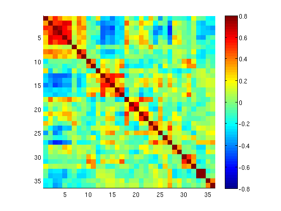
Seed-based correlation
After preprocessing, we can now generate a seed-to-seed correlation matrix for our subject.
If you look at the docs for seed_correl_161012.csh, you’ll see that we only need to add which regions to analyze (ROIs) to our instructions file.
Here we’ll use the canonical ROI list from $REFDIR as our input. You can use a different list of ROIS (i.e. BigBrain264,
BigBrain305), but there are a few things to be aware of:
ROIlistfile should contain only a single column
The single column should contain just the ROI file names. If you have additional columns (i.e. listing the coordinates), paste_4dfp will misinterpret them and cause the script to error. You can use the following command to create a file with just the first column:
cat $ROIlistfile | awk '{print $1}' > ${ROIlistfile}_1col.txt
The correlation matrix will not get generated if you have more than 256 ROIs
covariance used to only support up to 256 ROIs, so
seed_correlchecks for this and skips the correlation matrix step. Whilecovariancehas been updated to support more ROIs,seed_correlhas not. If you are using an ROI list with greater than 256 ROIs, you will run the following commands (after you runseed_correl) to get the correlation matrix (and remove intermediate files):# from $FCdir covariance -uom0 <patid>[_faln_dbnd]_xr3d_uwrp_atl.format <patid>_seed_regressors.dat /bin/rm *_ROI*_CCR.dat
# BOLD variables
set inpath = /path/to/project/${patid}
set target = $REFDIR/TRIO_KY_NDC
set go = 1
set sorted = 1
set economy = 0
set epi2atl = 1
set normode = 0

set nx = 90
set ny = 90

set skip = 0

set FDthresh = 0.2
set FDtype = 1
set anat_aveb = 10 # use 10mm preblur (voxel size < 3mm)

set TR_vol = 1.23
set TR_slc = 0 # use default (TR_vol/nslices)
set epidir = 0
set MBfac = 4
set seqstr = 1,8,15,6,13,4,11,2,9,16,7,14,5,12,3,10 # non-standard interleaving
set lomotil = 2 # filter FD in phase-encoding direction

set TE_vol = 33
set dwell = .59
set ped = y-
set rsam_cmnd = one_step_resample.csh

# fcMRI pre-processing
set srcdir = $cwd
set FSdir = /path/to/project/freesurfer/${patid}
set fcbolds = ( ${irun} )
set CSF_lcube = 3
set CSF_sd1t = 25
set CSF_svdt = .2
set WM_lcube = 5
set WM_svdt = .15
set bpss_params = ( -bh0.1 -oh2 )
set blur = .73542

# seed_correl ROIs
set ROIdir = ${REFDIR}/CanonicalROIsNP705
set ROIlistfile = ${REFDIR}/CanonicalROIsNP705/CanonicalROIsNP705.lst
Now we can go ahead and run it:
$ seed_correl_161012.csh NEWT002_s1.params ../NEWT_study.params
This produces a correlation matrix, ${FCdir}/${patid}_seed_regressors_CCR.dat.
You can display the matrix with any plotting tool (i.e. imagesc in matlab, matplotlib.pyplot.imshow in python).